Understanding temporal behavior is critical when designing systems where milliseconds matter. In the domain of embedded engineering and concurrent processing, a static representation of object interaction often fails to capture the nuances of execution speed and deadlines. This is where the UML timing diagram serves as an indispensable asset. It provides a precise visual mechanism for analyzing state changes and message exchanges over time.
This guide explores the mechanics, syntax, and practical application of timing diagrams. It is designed for developers who require clarity on latency, jitter, and state transitions without relying on marketing fluff. We will examine how to construct these diagrams, interpret complex constraints, and leverage them for safety-critical system verification.
🔍 What is a Timing Diagram?
A timing diagram is a specialized form of interaction diagram within the Unified Modeling Language (UML). Unlike sequence diagrams, which focus on the logical order of messages, timing diagrams emphasize the exact temporal relationships between events. They map the state of objects or lifelines against a time axis.
- Temporal Precision: They allow for the specification of absolute time (e.g., 50ms) or relative time (e.g., 10 units after event A).
- State Visibility: They explicitly show how long an object remains in a specific state.
- Concurrency: They illustrate how multiple processes operate simultaneously without collision.
For real-time developers, this distinction is vital. A system might function logically correctly but fail due to a missed deadline. A timing diagram helps visualize that failure before code is written.
🧩 Core Components and Syntax
To utilize this modeling technique effectively, one must understand its fundamental building blocks. Every diagram consists of a coordinate system defined by time and state.
1. Lifelines
Lifelines represent the existence of an object, process, or thread over a duration. They are drawn as vertical lines.
- Vertical Axis: Represents different entities or components.
- Horizontal Axis: Represents the progression of time.
- Activation Bars: Rectangles placed on the lifeline indicate when an object is actively performing an operation or is in a specific state.
2. State Boxes
State boxes are rectangular regions along a lifeline that denote the condition of the object. A transition from one state to another is marked by a boundary line.
- Occupied State: Indicates the object is processing or holding a resource.
- Idle State: Indicates the object is waiting or inactive.
- Labeling: States should be named clearly (e.g., Processing, Waiting, Blocked).
3. Time Axis Constraints
Time is not always linear in real-time systems. Constraints can define boundaries for events.
- Delay Constraints: Specify a minimum time before an event can occur.
- Deadline Constraints: Specify the maximum time allowed for an event completion.
- Periodicity: Define recurring events at fixed intervals.
⏱️ Visualizing State Changes
The primary value of a timing diagram lies in its ability to depict state transitions. In a sequence diagram, you see that message A was sent before message B. In a timing diagram, you see that the system was in State X for 10 milliseconds before transitioning to State Y.
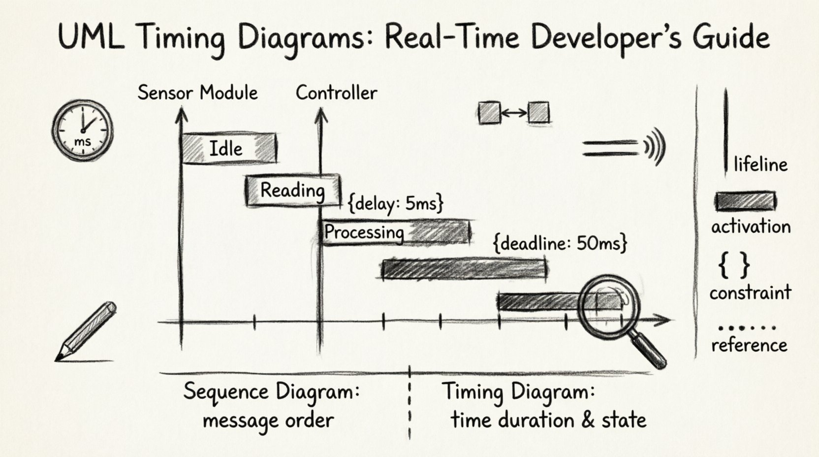
Consider a sensor reading loop. The system cycles through Idle, Reading, and Processing.
- Idle: The CPU waits for a trigger. Duration is variable.
- Reading: The hardware is active. Duration is fixed by hardware specs.
- Processing: The algorithm runs. Duration depends on data size.
By mapping these durations, a developer can identify bottlenecks. If the Processing state exceeds the deadline for the next Idle cycle, the system risks data loss.
🔒 Timing Constraints and Expressions
Real-time systems often require strict adherence to time limits. UML allows for the notation of these constraints using text labels or specific expressions attached to the diagram elements.
1. Absolute Time
Using absolute time anchors the diagram to a specific start point. For example, an event must occur at time t=100ms.
- Use case: Synchronization with an external clock source.
- Benefit: Ensures coordination across distributed components.
2. Relative Time
Relative time defines intervals based on previous events. For example, “Event B occurs 50ms after Event A”.
- Use case: Handling interrupt latencies.
- Benefit: Abstracts the diagram from the specific start time, focusing on flow.
3. Inequalities
Constraints can be expressed as inequalities, such as t < 50ms. This indicates a hard deadline.
- Hard Deadline: Failure to meet this results in system failure.
- Soft Deadline: Performance degrades if missed, but the system continues.
🔄 Concurrency and Parallelism
Modern software rarely runs on a single thread. Timing diagrams excel at showing parallel execution paths. When multiple lifelines exist, their horizontal progression indicates simultaneous activity.
1. Interleaving
Interleaving occurs when tasks share a single processor. The diagram shows slices of execution time for different tasks.
- Preemptive: A high-priority task interrupts a low-priority one.
- Non-Preemptive: Tasks run to completion before switching.
2. Resource Contention
When two lifelines require the same resource, one must wait. The diagram visualizes the wait time as a gap in the activation bar.
- Locking: One lifeline holds a resource while another waits.
- Deadlocks: If two lifelines wait for each other indefinitely, the diagram will show a continuous state of waiting.
⚖️ Timing Diagram vs. Sequence Diagram
Both diagrams model interactions, but their focus differs significantly. Confusing them can lead to design errors.
| Feature | Sequence Diagram | Timing Diagram |
|---|---|---|
| Primary Focus | Order of messages | Time duration and state |
| Time Axis | Implicit (logical order) | Explicit (quantitative) |
| State Representation | Minimal or implied | Detailed and explicit |
| Use Case | Logic flow, protocol design | Latency analysis, scheduling |
| Complexity | High for complex logic | High for timing precision |
Developers often use sequence diagrams for the initial logic design and timing diagrams for the subsequent real-time verification. This two-step approach ensures both correctness and performance.
🛠️ Construction Guidelines
Creating a useful diagram requires discipline. A cluttered diagram obscures the timing data it is meant to convey.
1. Define the Time Scale
Before drawing, decide on the unit of measurement. Is it milliseconds, CPU cycles, or abstract ticks? Consistency is key. Mixing units leads to confusion.
2. Group Related Activities
Group lifelines that belong to the same subsystem. Use boxes or frames to visually separate modules. This reduces cognitive load.
3. Label Constraints Clearly
Do not bury time constraints in small text. Place them near the relevant activation bar or message arrow. Use standard notation like {delay: 5ms}.
4. Simplify State Boxes
Do not show every micro-state. Focus on states that impact timing. If a state has negligible duration, merge it with the surrounding activity.
5. Validate with Data
Ensure the time values are not guesses. They should be derived from profiling data, hardware specifications, or worst-case execution time (WCET) analysis.
🚨 Common Pitfalls and Challenges
Even experienced engineers encounter difficulties when modeling time. Recognizing these pitfalls early prevents rework.
1. Over-Complication
Attempting to model the entire system in one diagram is a common error. A single diagram should focus on a specific interaction or subsystem. Break complex systems into smaller timing views.
2. Ignoring Jitter
Jitter is the variation in latency. A timing diagram often shows the ideal path. However, real systems have variance. Consider adding a range (e.g., 10ms ± 2ms) to represent jitter.
3. Static vs. Dynamic
Timing diagrams are often static representations of dynamic behavior. They do not account for runtime exceptions unless explicitly modeled. Ensure your diagram covers error handling scenarios.
4. Tooling Limitations
While many tools exist, some struggle with complex time constraints. Ensure the modeling environment supports the specific notation you need, such as nested constraints or non-linear time axes.
📊 Reference: Common Notation Symbols
Refer to this table for standard symbols used in timing diagrams.
| Symbol | Meaning |
|---|---|
| Vertical Line | Lifeline (Object/Thread) |
| Rectangular Bar on Line | Activation or State |
| Arrow with Label | Message or Signal |
| Box with Text | State Description |
| Brackets with Text | Constraint (e.g., delay, deadline) |
| Dashed Line | Reference or Link |
| Time Axis Tick | Time Unit Marker |
🧠 Deep Dive: Real-Time System Analysis
For developers in embedded systems, the timing diagram is more than a drawing; it is a contract. It defines the expected behavior of the hardware and software under specific conditions.
1. Interrupt Latency
Interrupts disrupt normal flow. A timing diagram helps calculate the maximum time between an interrupt signal and the start of the interrupt service routine (ISR).
- Context Switching: Time taken to save registers.
- Dispatch Time: Time to find the ISR handler.
- Execution: Time to run the handler code.
2. Bus Contention
In multi-core systems, the shared bus can become a bottleneck. The diagram shows when components access the bus and how long they hold it.
- Arbitration: Who gets access first?
- Wait States: How long does a component wait for the bus?
3. Power Management
Timing diagrams also help in power modeling. By knowing when the CPU is active versus idle, engineers can schedule low-power states.
- Idle Time: Window where power can be saved.
- Wake-up Time: Time required to return to full operation.
✅ Best Practices for Maintenance
Diagrams are living documents. As requirements change, the diagram must evolve.
- Version Control: Treat diagrams like code. Store them in a repository.
- Traceability: Link diagram elements to requirements. This ensures every time constraint is justified.
- Review Cycles: Include diagram reviews in the design phase. Peers can spot timing conflicts that the primary designer might miss.
- Automation: Where possible, generate test cases from the diagram to verify timing behavior automatically.
📝 Summary of Key Takeaways
The UML timing diagram offers a rigorous method for visualizing temporal relationships in software and hardware systems. It bridges the gap between logical flow and physical reality.
- Focus on Time: Use it when duration matters, not just order.
- Define Constraints: Clearly mark deadlines and delays.
- Visualize State: Show how long objects remain in specific conditions.
- Handle Concurrency: Map parallel execution paths to find contention points.
- Iterate: Refine the diagram as profiling data becomes available.
By integrating timing diagrams into the development lifecycle, teams can reduce the risk of real-time failures. This approach moves beyond theoretical correctness to practical performance assurance. It ensures that the system behaves not just as intended, but within the strict boundaries of its environment.
For those working on safety-critical applications, such as automotive control or medical devices, this level of detail is non-negotiable. It provides the evidence needed to validate that the system will meet its temporal requirements under all expected conditions.
Adopting this practice requires effort and discipline. However, the payoff is a system that is predictable, reliable, and performant. In the world of real-time development, predictability is the highest form of reliability.