


Designing high-performance systems requires precision. When modeling interactions within complex software architectures, the choice of diagram type dictates the clarity of the analysis. The decision often lies between the UML Sequence Diagram and the UML Timing Diagram. While Sequence Diagrams excel at illustrating logical flow, Timing Diagrams offer granular control over temporal constraints. Understanding the distinction is critical for engineers tasked with latency optimization, real-time system verification, and concurrency management.
This guide explores the technical nuances of switching from Sequence to Timing models. It details when temporal fidelity outweighs interaction logic and how to model performance metrics effectively without relying on proprietary tools. We will examine the structural differences, specific use cases, and the modeling implications for system reliability.
Understanding Sequence Diagrams in Performance Contexts ⏱️
Sequence Diagrams are the industry standard for modeling object interactions over time. They focus on the order of messages passed between lifelines. In a typical performance review, engineers use these diagrams to trace the path of a request through a system.
Strengths of Sequence Modeling
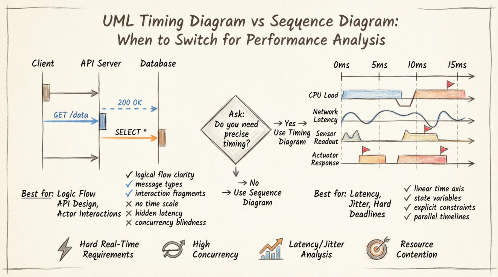
- Logical Flow Clarity: They clearly show which component calls which, making the control flow easy to understand.
- Message Types: They distinguish between synchronous calls, asynchronous signals, and return messages visually.
- Interaction Fragments: They support
alt,opt, andloopfragments to model conditional logic and iterations. - Actor Representation: They are excellent for showing external user or system triggers initiating processes.
Limitations for Performance Analysis
Despite their popularity, Sequence Diagrams have inherent limitations when used for strict performance analysis. The time axis in a Sequence Diagram is relative, not absolute. It implies sequence but does not strictly quantify duration.
- Absence of Time Scale: There is no horizontal time axis. The distance between messages is arbitrary and does not represent milliseconds or seconds.
- Hidden Latency: While activation bars show duration, they do not easily accommodate overlapping events on the same lifeline unless the diagram becomes cluttered.
- Concurrency Blindness: Modeling parallel execution paths is difficult. Overlapping activations can imply concurrency, but exact timing relationships are hard to define.
- Constraint Complexity: Adding timing constraints (e.g., “response must be under 50ms”) requires text notes, which are often overlooked during visual reviews.
When performance requirements become strict, such as in embedded systems or high-frequency trading platforms, the ambiguity of the Sequence Diagram becomes a liability. Engineers need to know not just what happens, but exactly when it happens relative to the clock.
The Case for Timing Diagrams 📊
The UML Timing Diagram provides a specialized view where the horizontal axis represents time. This shift from interaction order to temporal progression allows for the precise modeling of state changes and deadlines.
Core Capabilities for Performance
- Linear Time Axis: A defined scale (e.g., microseconds, milliseconds) allows for direct measurement of intervals.
- State Variables: Diagrams can track the state of specific variables (e.g., `cpu_load`, `queue_depth`) over time, not just object activation.
- Timing Constraints: Explicit annotations define minimum, maximum, and exact durations for transitions.
- Parallelism: Multiple state changes can be visualized simultaneously on different lifelines, making concurrency visible.
Visualizing Real-Time Behavior
Real-time systems often operate under hard or soft deadlines. A Timing Diagram allows engineers to map these deadlines directly against the execution timeline. If a task must complete within 10ms, the diagram can show the start time, the duration of the task, and the deadline marker.
This visualization helps identify bottlenecks that Sequence Diagrams might hide. For instance, a sequence of three calls might appear sequential in a Sequence Diagram. In a Timing Diagram, if two calls happen in parallel on different cores, the total duration is reduced. The Timing Diagram captures this optimization explicitly.
Comparative Analysis: Sequence vs. Timing 📋
To understand the trade-offs, we can compare the two modeling approaches across several dimensions. The following table outlines the structural and functional differences.
| Feature | Sequence Diagram | Timing Diagram |
|---|---|---|
| Primary Focus | Order of interactions | Duration of states |
| Time Representation | Relative / Implicit | Absolute / Explicit Scale |
| Lifelines | Objects / Components | Objects / Variables / Clocks |
| State Visibility | Activation Bars | State Invariants / Signal Values |
| Concurrency | Overlapping Bars | Parallel Timelines |
| Best Use Case | Logic Flow / API Design | Latency / Jitter / Deadlines |
| Complexity | Low to Medium | Medium to High |
As the table indicates, the choice depends on the specific question being asked. If the question is “Does component A call component B before C?”, use Sequence. If the question is “Does component A complete before the deadline at 500ms?”, use Timing.
Decision Framework: When to Switch 🔄
Switching from a Sequence focus to a Timing focus is not a binary decision but a progression based on system requirements. Below are specific scenarios that necessitate a switch.
1. Hard Real-Time Requirements
Systems that must respond within a guaranteed timeframe (e.g., automotive braking systems, medical devices) require Timing Diagrams. Sequence diagrams cannot enforce the temporal boundaries required for certification. The Timing Diagram allows for the definition of timingConstraint elements that verify the system meets safety standards.
2. High Concurrency Environments
In multi-threaded or distributed systems, the order of events may vary, but the timing relationship must remain consistent. A Timing Diagram can show that while Thread A and Thread B run concurrently, Thread A must not exceed a specific duration before Thread B proceeds. Sequence diagrams often assume a strict ordering that does not exist in true parallel architectures.
3. Latency and Jitter Analysis
Jitter is the variation in latency over time. Sequence diagrams show a single path. Timing diagrams can show multiple paths with varying durations to represent jitter. If performance analysis requires understanding the variance in response time (e.g., 95th percentile latency), the Timing Diagram is the appropriate tool.
4. Resource Contention Modeling
When modeling resource contention, such as CPU usage or memory bandwidth, Timing Diagrams are superior. They can display state variables representing resource availability. Engineers can visualize when a resource is busy versus idle, allowing for better capacity planning.
Modeling Performance Metrics Deep Dive 📏
Once the switch to Timing Diagrams is made, the focus shifts to specific metrics. These metrics must be modeled accurately to ensure the diagram reflects reality.
Latency
Latency is the total time from request initiation to response completion. In a Timing Diagram, this is the interval between the trigger event on the first lifeline and the return event on the last lifeline. To model this:
- Mark the start time of the trigger event.
- Mark the end time of the final response event.
- Use a constraint annotation to define the maximum allowable interval.
Throughput
Throughput measures the number of events processed per unit of time. Modeling throughput in a Timing Diagram involves repeating patterns. Use loop fragments or repetition markers to indicate a steady stream of requests. The density of events along the time axis visually represents throughput.
Deadlines and Timeouts
Deadlines are critical in performance modeling. A Timing Diagram can include a vertical dashed line representing a deadline. If a process state extends past this line, it indicates a violation. This visual cue is more immediate than reading a textual constraint in a Sequence Diagram.
Jitter and Variance
Jitter is represented by the inconsistency in the intervals between events. If a periodic task should fire every 10ms, but the actual time varies between 9ms and 12ms, the Timing Diagram can show this variance. This is crucial for audio/video streaming systems or network packet processing.
Technical Elements of Timing Diagrams 🔧
To use Timing Diagrams effectively, one must understand the specific UML elements involved. These elements differ from standard Sequence Diagram notation.
State Variables
Unlike Sequence Diagrams which focus on object lifelines, Timing Diagrams often focus on state variables. A variable might be modeled as a lifeline where the state changes are represented by steps. For example, a variable temperature might have a state transition from normal to critical at a specific time point.
Timing Constraints
These are annotations attached to transitions or events. They define the temporal relationship. Common constraints include:
- minimum: The earliest time an event can occur.
- maximum: The latest time an event must occur.
- exact: A precise time point for an event.
- range: A window of time during which an event must occur.
Signal Values
Timing Diagrams can display the value of signals over time. This is useful for monitoring bus loads or data rates. A continuous line might represent a signal value, with vertical steps indicating changes in the data stream.
Common Modeling Mistakes ⚠️
Transitioning to Timing Diagrams introduces new complexities. Engineers often fall into traps that reduce the utility of the model.
1. Over-Modeling Static Logic
Not every interaction requires a Timing Diagram. If the logic is purely sequential and timing is irrelevant, a Timing Diagram adds unnecessary complexity. Reserve them for performance-critical paths.
2. Ignoring Clock Domains
In distributed systems, different components may operate on different clock domains. A Timing Diagram assumes a synchronized time axis. If components are asynchronous, the diagram must account for clock skew or use separate timelines with synchronization points.
3. Ambiguous Scale Units
Always define the time scale clearly (e.g., ms, µs, ns). Mixing units without clear labels leads to misinterpretation. A scale of 100 might mean 100 milliseconds or 100 nanoseconds. Clarity is paramount.
4. Neglecting Idle Times
Performance is often defined by what happens when the system is idle. Timing Diagrams should show periods of inactivity to calculate utilization rates. Ignoring idle time can lead to overestimating system capacity.
Integration with System Architecture 🏗️
Timing Diagrams do not exist in isolation. They must integrate with the broader system architecture documentation.
Linking to Deployment Diagrams
The lifelines in a Timing Diagram should correspond to physical nodes or logical partitions defined in the Deployment Diagram. This ensures that the timing analysis reflects the actual hardware or network topology. For example, a delay between two lifelines should correspond to network latency between the servers they represent.
Traceability to Requirements
Each timing constraint in the diagram should trace back to a non-functional requirement. This traceability is essential for verification and validation. If a requirement states “System must respond in 200ms,” the Timing Diagram must explicitly show this constraint and the actual modeled duration.
Maintenance and Evolution 🔄
As systems evolve, Timing Diagrams require maintenance. Performance characteristics change with updates, load changes, and infrastructure shifts.
- Version Control: Treat Timing Diagrams as code. Store them in version control systems to track changes in timing constraints over releases.
- Performance Profiling: Update diagrams based on actual profiling data. If a component takes longer in production than modeled, update the constraint to reflect reality.
- Scenario Updates: New features introduce new timing paths. Ensure all critical paths are updated to avoid gaps in analysis.
Best Practices for Performance Modeling ✅
To maximize the value of Timing Diagrams, follow these established practices.
- Keep Lifelines Simple: Avoid too many lifelines. Focus on the critical path. Group related components if necessary.
- Use Standard Notation: Adhere to UML 2.5 standards for constraints and lifelines to ensure consistency across the team.
- Highlight Critical Paths: Use color or bolding to indicate the paths that determine the overall system performance.
- Document Assumptions: Note any assumptions made about network speed or processing power. These assumptions affect the validity of the timing analysis.
- Review Regularly: Schedule reviews of Timing Diagrams during design iterations. Early detection of timing violations saves significant refactoring effort later.
Final Considerations for Engineering Teams 👥
Selecting the right modeling notation is a strategic decision. Sequence Diagrams remain the default for logic and flow. Timing Diagrams are the specialized tool for temporal precision. The choice should not be arbitrary.
Teams should assess their performance requirements before committing to a modeling strategy. If the system is latency-sensitive, the overhead of creating Timing Diagrams is justified by the reduction in risk. If the system is primarily business-logic driven, Sequence Diagrams remain sufficient.
Ultimately, the goal is clarity. Whether using Sequence or Timing, the diagram must communicate the system behavior accurately to stakeholders, developers, and testers. By understanding the specific strengths of the Timing Diagram, engineers can ensure that performance is not an afterthought but a core component of the design.